Package Imports
from io import BytesIO
from netrc import netrc
from pathlib import Path

import matplotlib.pyplot as plt
import numpy as np
import pandas as pd
import requests
import xarray as xr
from matplotlib.colors import ListedColormap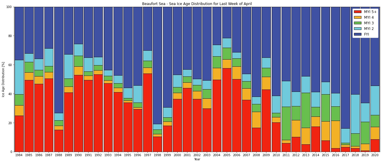
Checking out a really neat historical sea ice age dataset from NSIDC: https://nsidc.org/data/nsidc-0611
from io import BytesIO
from netrc import netrc
from pathlib import Path
import matplotlib.pyplot as plt
import numpy as np
import pandas as pd
import requests
import xarray as xr
from matplotlib.colors import ListedColormapWe need to get the data first (requires a NASA EarthData account!)
local_nc = Path('./iceage_nsidc.nc')
if local_nc.exists():
    ds = xr.open_dataset(
        local_nc
    ).chunk(
        {'time': 200, 'x': 722, 'y': 722} # try to have ~100MB chunks
    )
else:
    resp = input(
        'Local dataset does not exist - confirm you ' \
        'want to download from NSIDC? (Approx bandwidth usage: 1GB)'
    )
    if resp.lower() == 'y':
        base_url = 'https://daacdata.apps.nsidc.org/pub/DATASETS/' \
                   'nsidc0611_seaice_age_v4/data/' \
                   'iceage_nh_12.5km_{year}0101_{year}1231_v4.1.nc'
        urls = [
            base_url.format(year=y)
            for y in range(1984,2021)  # 2021 is still preliminary
        ]
        try:
            user, _, password = netrc().authenticators('urs.earthdata.nasa.gov')
        except KeyError:
            print("No EarthData entry in ~/.netrc")
            raise ValueError
        with requests.Session() as sesh:
            sesh.auth = (user, password)
            ds = xr.open_mfdataset(
                [
                    BytesIO(sesh.get(url).content)
                    for url in urls
                ],
                data_vars=['age_of_sea_ice']
            )
    else:
        raise FileNotFoundError(
            'Local dataset not found user decided not to download'
)ds<xarray.Dataset> Size: 1GB
Dimensions: (time: 1924, y: 722, x: 722)
Coordinates:
* time (time) object 15kB 1984-01-01 00:00:00 ... 2020-12-23 00:...
* y (y) float32 3kB -4.518e+06 -4.506e+06 ... 4.518e+06
* x (x) float32 3kB -4.518e+06 -4.506e+06 ... 4.518e+06
Data variables:
crs int32 4B ...
age_of_sea_ice (time, y, x) uint8 1GB dask.array<chunksize=(200, 722, 722), meta=np.ndarray>
latitude (y, x) float32 2MB dask.array<chunksize=(722, 722), meta=np.ndarray>
longitude (y, x) float32 2MB dask.array<chunksize=(722, 722), meta=np.ndarray>
Attributes:
version: 4.1
release_date: April 2019
Conventions: CF-1.4
citation: Tschudi, M. A., Meier, W. N., and Stewart, J. S.: An enhan...
dataset_doi: 10.5067/UTAV7490FEPBds['age_of_sea_ice']<xarray.DataArray 'age_of_sea_ice' (time: 1924, y: 722, x: 722)> Size: 1GB
dask.array<xarray-age_of_sea_ice, shape=(1924, 722, 722), dtype=uint8, chunksize=(200, 722, 722), chunktype=numpy.ndarray>
Coordinates:
* time (time) object 15kB 1984-01-01 00:00:00 ... 2020-12-23 00:00:00
* y (y) float32 3kB -4.518e+06 -4.506e+06 ... 4.506e+06 4.518e+06
* x (x) float32 3kB -4.518e+06 -4.506e+06 ... 4.506e+06 4.518e+06
Attributes:
short_name: ice age
long_name: age_of_sea_ice
standard_name: age_of_sea_ice
units: year
flag_values: [20 21]
grid_mapping: crs
comment: Ice of this age is up-to-this-number of years old. A val...print('Approximate size of uncompressed dataset: %.2f MB' % (
ds.nbytes / 1024**2
))Approximate size of uncompressed dataset: 960.49 MBHere we take a single time slice and try to figure out the best way to get a Beaufort-Only subset
time_slice = ds.isel(time=1200)
time_slice['age_of_sea_ice']
<xarray.DataArray 'age_of_sea_ice' (y: 722, x: 722)> Size: 521kB
dask.array<getitem, shape=(722, 722), dtype=uint8, chunksize=(722, 722), chunktype=numpy.ndarray>
Coordinates:
* y (y) float32 3kB -4.518e+06 -4.506e+06 ... 4.506e+06 4.518e+06
* x (x) float32 3kB -4.518e+06 -4.506e+06 ... 4.506e+06 4.518e+06
time object 8B 2007-01-29 00:00:00
Attributes:
short_name: ice age
long_name: age_of_sea_ice
standard_name: age_of_sea_ice
units: year
flag_values: [20 21]
grid_mapping: crs
comment: Ice of this age is up-to-this-number of years old. A val...time_slice['age_of_sea_ice'].plot(add_colorbar=False);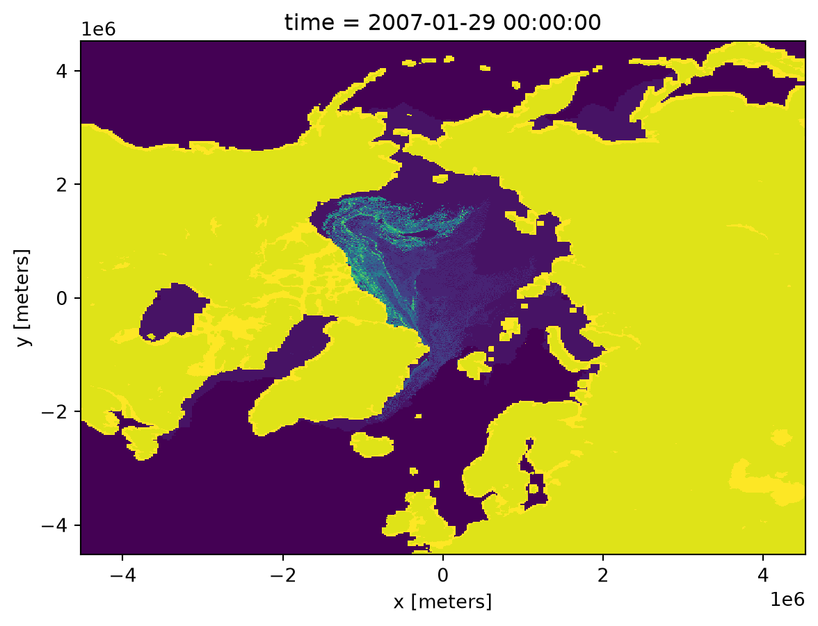
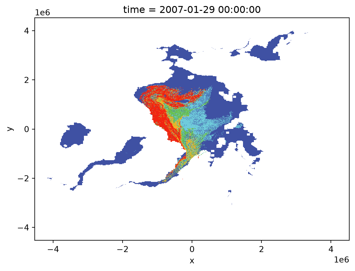
Let’s plot with the NSIDC colormap
# this implementation is imperfect but seems to work okay
cmap = ListedColormap(
    [
        '#FFFFFF', '#3F51A3', '#6FCBDB', '#69BF4E', '#F3B226',
        '#F12411', '#F12411', '#F12411', '#F12411', '#F12411',
        '#F12411', '#F12411', '#F12411', '#F12411', '#F12411',
        '#F12411'
    ],
    name='Sea Ice Age'
)
cmap.set_over('#A1A1A1')
cmap
# note how we mask out the land/channels with a nice little conditional
xr.where(
    time_slice['age_of_sea_ice'] >= 20,
    np.nan,
    time_slice['age_of_sea_ice']
).plot(
    cmap=cmap,
    add_colorbar=False
);
Create a Mask based on Dave’s Figure 1B: https://doi.org/10.1002/essoar.10509833.1
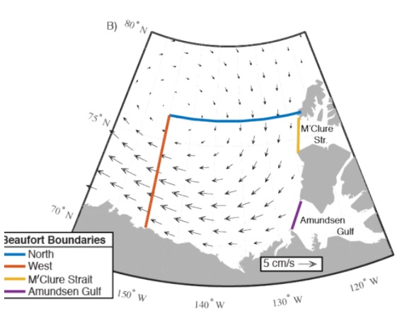
# approximate bounding box
min_lon = -150
max_lon = -120
min_lat = 68
max_lat = 76
lons = time_slice['longitude'].data.copy()
lons[lons < min_lon] = np.nan
lons[lons > max_lon] = np.nan
lons[~np.isnan(lons)] = 1
lats = time_slice['latitude'].data.copy()
lats[lats > max_lat] = np.nan
lats[lats < min_lat] = np.nan
lats[~np.isnan(lats)] = 1
mask = lons * lats
fig, (
    (ax_lons, ax_lats), (ax_mask, ax_data)
) = plt.subplots(ncols=2, nrows=2)
ax_lons.imshow(lons, origin='lower')
ax_lons.set_title('Beaufort Lon mask\n(>= -150 and <= -120)')
ax_lats.imshow(lats, origin='lower')
ax_lats.set_title('Beaufort Lat mask\n(>= 68 and <=76)')
ax_mask.imshow(mask, origin='lower')
ax_mask.imshow(lons, origin='lower', cmap='Greens_r', alpha=0.4, zorder=-2)
ax_mask.imshow(lats, origin='lower', cmap='Blues_r', alpha=0.4, zorder=-2)
ax_mask.set_title('Beaufort mask (lon * lat)')
ax_mask.set_xlim(150, 350)
ax_mask.set_ylim(375, 575)
ax_data.imshow(time_slice['age_of_sea_ice'] * mask, cmap=cmap, vmin=0, vmax=16)
ax_data.set_title('Masked Ice Age data')
ax_data.set_xlim(150, 350)
ax_data.set_ylim(375, 575)
fig.tight_layout();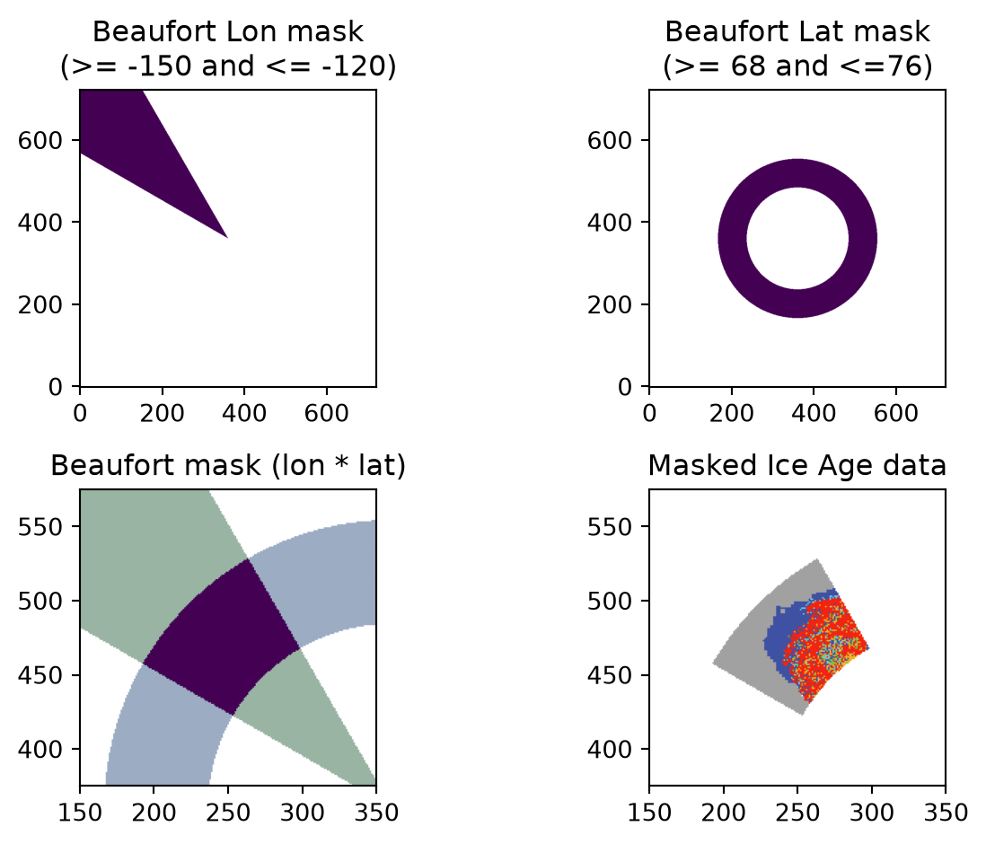
Let’s also reduce our spatial grid size to further minimize the footprint of the masked dataset
# just eyeballed these based on the above figure
xs = xr.DataArray(range(220, 300), dims='x')
ys = xr.DataArray(range(415, 535), dims='y')
(time_slice['age_of_sea_ice'] * mask).isel(
    x=xs, y=ys
).plot(cmap=cmap, vmin=0, vmax=16, add_colorbar=False);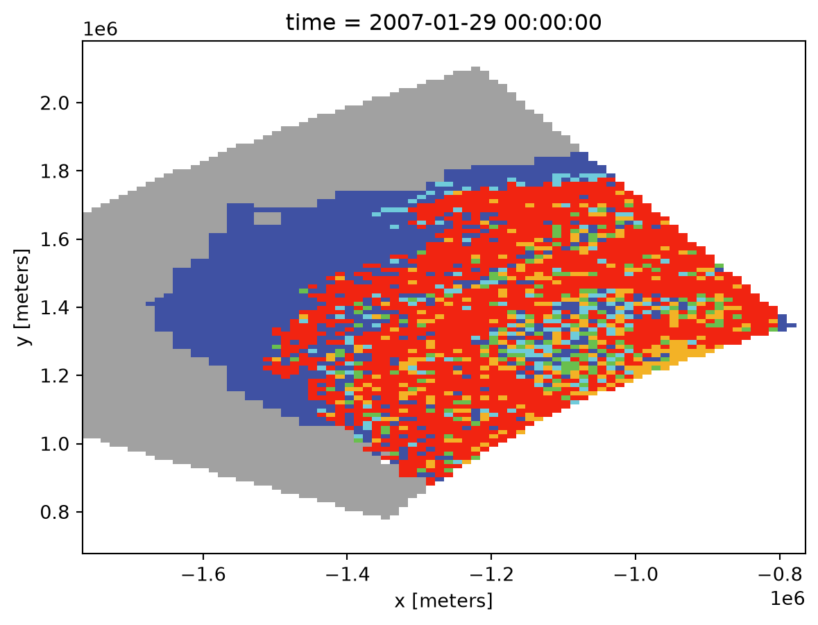
Now that we have our slicers we can reduce the dataset to just the Beaufort AOI
result = (ds['age_of_sea_ice'].isel(x=xs, y=ys) * mask[415:535, 220:300])
result
<xarray.DataArray (time: 1924, y: 120, x: 80)> Size: 74MB
dask.array<mul, shape=(1924, 120, 80), dtype=float32, chunksize=(200, 120, 80), chunktype=numpy.ndarray>
Coordinates:
* time (time) object 15kB 1984-01-01 00:00:00 ... 2020-12-23 00:00:00
* y (y) float32 480B 6.831e+05 6.956e+05 ... 2.162e+06 2.175e+06
* x (x) float32 320B -1.761e+06 -1.748e+06 ... -7.834e+05 -7.708e+05
Attributes:
short_name: ice age
long_name: age_of_sea_ice
standard_name: age_of_sea_ice
units: year
flag_values: [20 21]
grid_mapping: crs
comment: Ice of this age is up-to-this-number of years old. A val...print('Approximate size of minimized dataset: %.2f MB' % (
result.nbytes / 1024**2
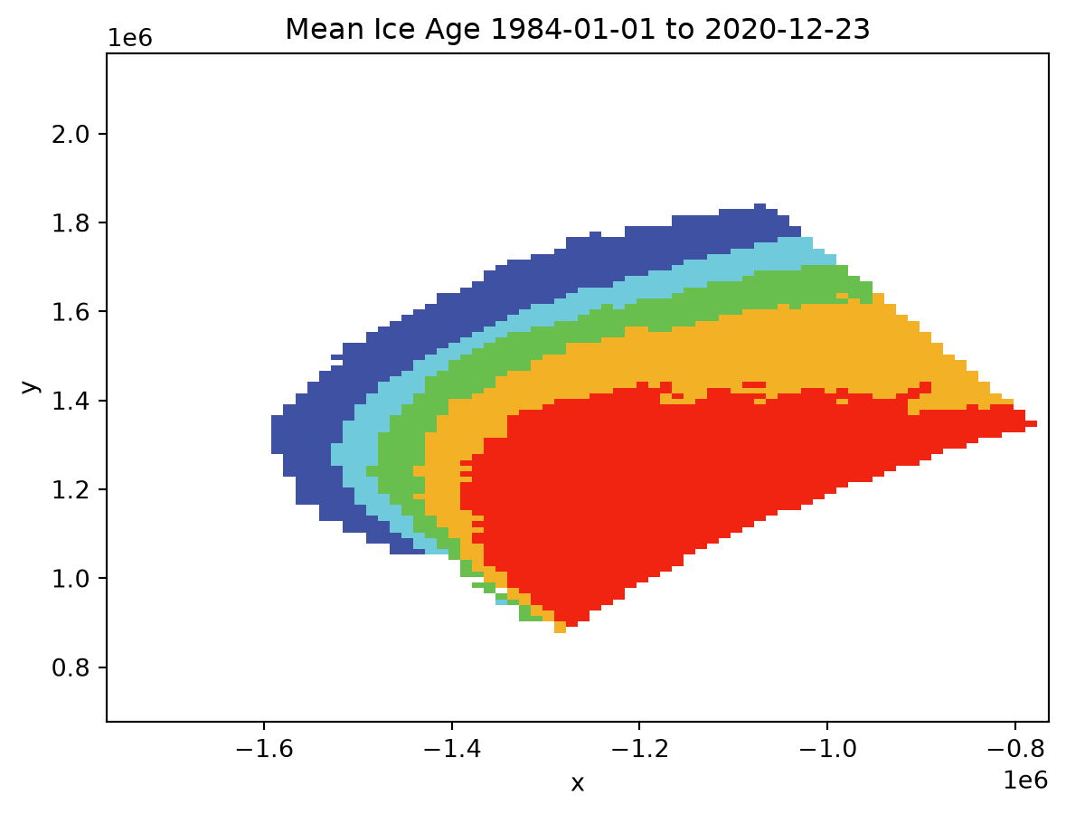
))Approximate size of minimized dataset: 70.46 MBfig, ax = plt.subplots()
xr.where(
result >= 20,
np.nan,
result
).mean(dim='time').plot(
cmap=cmap,
ax=ax,
vmin=0,
vmax=16,
add_colorbar=False
)
ax.set_title(
'Mean Ice Age ' +\
result["time"].min().dt.strftime("%Y-%m-%d").data +\
' to ' +\
result["time"].max().dt.strftime("%Y-%m-%d").data
);
# any ice age greater than 5 will be given the "5+" moniker
data = xr.where(result >= 20, np.nan, result)
data = xr.where(data > 5, 5, data)
# imperfect but works
last_week_apr = data.loc[
    (data['time'].dt.month == 4) &
    ((31 - data['time'].dt.day) < 5)
]
assert \
    len(last_week_apr['time']) == \
    len(range(
        data['time.year'].min().values,
        data['time.year'].max().values+1
    ))
last_week_apr
<xarray.DataArray (time: 37, y: 120, x: 80)> Size: 1MB dask.array<getitem, shape=(37, 120, 80), dtype=float32, chunksize=(37, 120, 80), chunktype=numpy.ndarray> Coordinates: * time (time) object 296B 1984-04-29 00:00:00 ... 2020-04-29 00:00:00 * y (y) float32 480B 6.831e+05 6.956e+05 ... 2.162e+06 2.175e+06 * x (x) float32 320B -1.761e+06 -1.748e+06 ... -7.834e+05 -7.708e+05
Now that we have our last-week-of-April timeseries we can construct a nice figure
# if it's stupid and it works - it's not stupid
df = pd.DataFrame({
    'Year': [],
    'FYI': [],
    'MYI 2': [],
    'MYI 3': [],
    'MYI 4': [],
    'MYI 5+': []
})
for year in last_week_apr['time.year'].values:
    flat = last_week_apr.isel(time=last_week_apr['time.year'].isin([year])).values.ravel()
    vals, counts = np.unique(flat[~np.isnan(flat)], return_counts=True)
    if vals[0] != 0:
        df = pd.concat([
                df,
                pd.DataFrame({
                    'Year': [year],
                    'FYI': [counts[0]],
                    'MYI 2': [counts[1]],
                    'MYI 3': [counts[2]],
                    'MYI 4': [counts[3]],
                    'MYI 5+': [counts[4]]
                })
            ],
            ignore_index=True
        )
    else:
        df = pd.concat([
                df,
                pd.DataFrame({
                    'Year': [year],
                    'FYI': [counts[1]],
                    'MYI 2': [counts[2]],
                    'MYI 3': [counts[3]],
                    'MYI 4': [counts[4]],
                    'MYI 5+': [counts[5]]
                })
            ],
            ignore_index=True
        )
df = df.set_index(df['Year'].astype('uint32')).drop('Year', axis=1)

# convert pixel counts into fraction of total
totals = df.sum(axis=1) / 100
for col in df.columns:
    df[col] /= totals

# put it all together
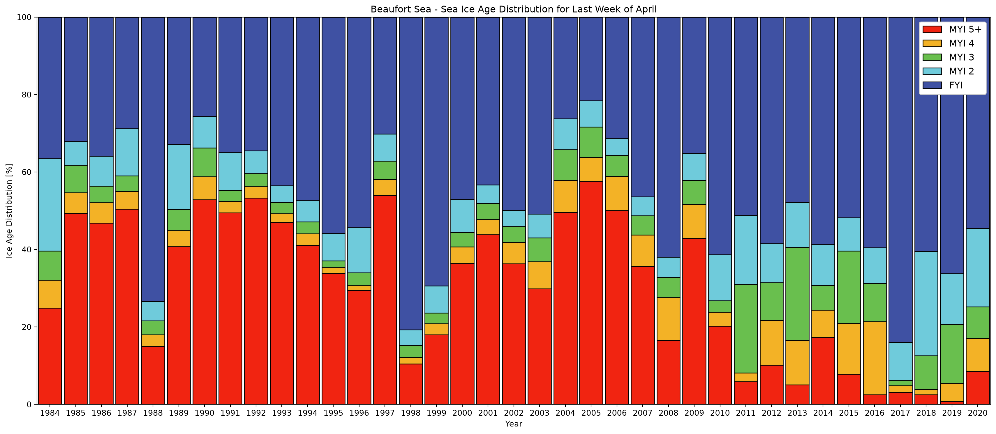
fig, ax = plt.subplots(figsize=(22,9))
# need to invert column order to match dave's figure 3c
df[df.columns[::-1]].plot(
    kind='bar',
    stacked=True,
    ax=ax,
    width=0.9,
    color=['#3F51A3', '#6FCBDB', '#69BF4E', '#F3B226', '#F12411'][::-1],
    edgecolor='k'
)
ax.set_xlim(-0.5, len(df)-0.5)
ax.set_ylim(0, 100)
ax.set_ylabel('Ice Age Distribution [%]')
ax.legend(framealpha=1, loc='upper right', fontsize=12)
[lab.set_rotation(0) for lab in ax.get_xticklabels()]
ax.set_title('Beaufort Sea - Sea Ice Age Distribution for Last Week of April');